optimal performance - traduzione in russo
Diclib.com
Dizionario ChatGPT
Inserisci una parola o una frase in qualsiasi lingua 👆
Lingua:

Traduzione e analisi delle parole tramite l'intelligenza artificiale ChatGPT

In questa pagina puoi ottenere un'analisi dettagliata di una parola o frase, prodotta utilizzando la migliore tecnologia di intelligenza artificiale fino ad oggi:

  • come viene usata la parola
  • frequenza di utilizzo
  • è usato più spesso nel discorso orale o scritto
  • opzioni di traduzione delle parole
  • esempi di utilizzo (varie frasi con traduzione)
  • etimologia

optimal performance - traduzione in russo

MAXIMIZED OBJECTIVE FUNCTION OF AN OPTIMIZATION PROBLEM
Optimal value function; Cost-to-go function; Optimal performance function

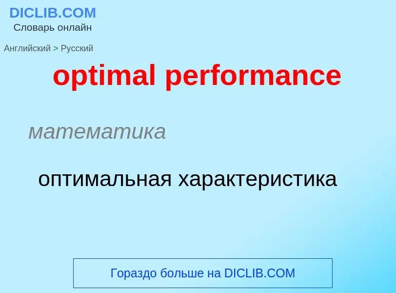
optimal performance      

математика

оптимальная характеристика

optimal stopping problem         
CLASS OF MATHEMATICAL PROBLEMS CONCERNED WITH CHOOSING AN OPTIMAL TIME TO TAKE A PARTICULAR ACTION
Optimal Stopping; Optimal Stopping problem
задача об оптимальной остановке
optimal experiment         
EXPERIMENTAL DESIGN THAT IS OPTIMAL WITH RESPECT TO SOME STATISTICAL CRITERION
Optimum design; Optimum experiment; Optimal experiment; Optimum experimental designs; Model-oriented design of experiments; Optimal Design of Experiments; Alphabetic optimality; Optimal design of experiments; Optimal design of experiment; Optimum design of experiments; Optimum design of experiment; Optimal experimental design; Optimum experimental design; Optimal experimental designs; D-optimal design; E-optimal design; Optimal design model selection

математика

оптимальный эксперимент

Definizione

PERFORM
<programming> A COBOL statement used for executing "paragraphs". [What's a paragraph?] (1997-06-10)

Wikipedia

Value function

The value function of an optimization problem gives the value attained by the objective function at a solution, while only depending on the parameters of the problem. In a controlled dynamical system, the value function represents the optimal payoff of the system over the interval [t, t1] when started at the time-t state variable x(t)=x. If the objective function represents some cost that is to be minimized, the value function can be interpreted as the cost to finish the optimal program, and is thus referred to as "cost-to-go function." In an economic context, where the objective function usually represents utility, the value function is conceptually equivalent to the indirect utility function.

In a problem of optimal control, the value function is defined as the supremum of the objective function taken over the set of admissible controls. Given ( t 0 , x 0 ) [ 0 , t 1 ] × R d {\displaystyle (t_{0},x_{0})\in [0,t_{1}]\times \mathbb {R} ^{d}} , a typical optimal control problem is to

maximize J ( t 0 , x 0 ; u ) = t 0 t 1 I ( t , x ( t ) , u ( t ) ) d t + ϕ ( x ( t 1 ) ) {\displaystyle {\text{maximize}}\quad J(t_{0},x_{0};u)=\int _{t_{0}}^{t_{1}}I(t,x(t),u(t))\,\mathrm {d} t+\phi (x(t_{1}))}

subject to

d x ( t ) d t = f ( t , x ( t ) , u ( t ) ) {\displaystyle {\frac {\mathrm {d} x(t)}{\mathrm {d} t}}=f(t,x(t),u(t))}

with initial state variable x ( t 0 ) = x 0 {\displaystyle x(t_{0})=x_{0}} . The objective function J ( t 0 , x 0 ; u ) {\displaystyle J(t_{0},x_{0};u)} is to be maximized over all admissible controls u U [ t 0 , t 1 ] {\displaystyle u\in U[t_{0},t_{1}]} , where u {\displaystyle u} is a Lebesgue measurable function from [ t 0 , t 1 ] {\displaystyle [t_{0},t_{1}]} to some prescribed arbitrary set in R m {\displaystyle \mathbb {R} ^{m}} . The value function is then defined as

with V ( t 1 , x ( t 1 ) ) = ϕ ( x ( t 1 ) ) {\displaystyle V(t_{1},x(t_{1}))=\phi (x(t_{1}))} , where ϕ ( x ( t 1 ) ) {\displaystyle \phi (x(t_{1}))} is the "scrap value". If the optimal pair of control and state trajectories is ( x , u ) {\displaystyle (x^{\ast },u^{\ast })} , then V ( t 0 , x 0 ) = J ( t 0 , x 0 ; u ) {\displaystyle V(t_{0},x_{0})=J(t_{0},x_{0};u^{\ast })} . The function h {\displaystyle h} that gives the optimal control u {\displaystyle u^{\ast }} based on the current state x {\displaystyle x} is called a feedback control policy, or simply a policy function.

Bellman's principle of optimality roughly states that any optimal policy at time t {\displaystyle t} , t 0 t t 1 {\displaystyle t_{0}\leq t\leq t_{1}} taking the current state x ( t ) {\displaystyle x(t)} as "new" initial condition must be optimal for the remaining problem. If the value function happens to be continuously differentiable, this gives rise to an important partial differential equation known as Hamilton–Jacobi–Bellman equation,

V ( t , x ) t = max u { I ( t , x , u ) + V ( t , x ) x f ( t , x , u ) } {\displaystyle -{\frac {\partial V(t,x)}{\partial t}}=\max _{u}\left\{I(t,x,u)+{\frac {\partial V(t,x)}{\partial x}}f(t,x,u)\right\}}

where the maximand on the right-hand side can also be re-written as the Hamiltonian, H ( t , x , u , λ ) = I ( t , x , u ) + λ f ( t , x , u ) {\displaystyle H\left(t,x,u,\lambda \right)=I(t,x,u)+\lambda f(t,x,u)} , as

V ( t , x ) t = max u H ( t , x , u , λ ) {\displaystyle -{\frac {\partial V(t,x)}{\partial t}}=\max _{u}H(t,x,u,\lambda )}

with V ( t , x ) / x = λ ( t ) {\displaystyle \partial V(t,x)/\partial x=\lambda (t)} playing the role of the costate variables. Given this definition, we further have d λ ( t ) / d t = 2 V ( t , x ) / x t + 2 V ( t , x ) / x 2 f ( x ) {\displaystyle \mathrm {d} \lambda (t)/\mathrm {d} t=\partial ^{2}V(t,x)/\partial x\partial t+\partial ^{2}V(t,x)/\partial x^{2}\cdot f(x)} , and after differentiating both sides of the HJB equation with respect to x {\displaystyle x} ,

2 V ( t , x ) t x = I x + 2 V ( t , x ) x 2 f ( x ) + V ( t , x ) x f ( x ) x {\displaystyle -{\frac {\partial ^{2}V(t,x)}{\partial t\partial x}}={\frac {\partial I}{\partial x}}+{\frac {\partial ^{2}V(t,x)}{\partial x^{2}}}f(x)+{\frac {\partial V(t,x)}{\partial x}}{\frac {\partial f(x)}{\partial x}}}

which after replacing the appropriate terms recovers the costate equation

λ ˙ ( t ) = I x + λ ( t ) f ( x ) x = H x {\displaystyle -{\dot {\lambda }}(t)={\frac {\partial I}{\partial x}}+\lambda (t){\frac {\partial f(x)}{\partial x}}={\frac {\partial H}{\partial x}}}

where λ ˙ ( t ) {\displaystyle {\dot {\lambda }}(t)} is Newton notation for the derivative with respect to time.

The value function is the unique viscosity solution to the Hamilton–Jacobi–Bellman equation. In an online closed-loop approximate optimal control, the value function is also a Lyapunov function that establishes global asymptotic stability of the closed-loop system.
Traduzione di &#39optimal performance&#39 in Russo